Signal Analysis

After detecting events, the next step is extracting quantitative features. ionique provides extract_features() to collect segment statistics into a pandas DataFrame, plus tools for IV curve analysis.

Segment statistics

Every segment (Segment or MetaSegment) exposes these computed properties:

event = trace.traverse_to_rank("event")[0]

event.mean      # mean current (nA)
event.std       # standard deviation
event.min       # minimum current value
event.max       # maximum current value
event.n         # number of samples
event.duration  # time in seconds (requires sampling_freq in tree)

These are computed from the underlying current array on each access.

Extracting features with extract_features

extract_features() walks the segment tree, collects statistics from every segment at a target rank, and returns a DataFrame:

from ionique.utils import extract_features

df = extract_features(
    trace,
    bottom_rank="event",
    extractions=["mean", "std", "min", "max", "duration", "n"],
)
print(df.head())
#       mean      std      min      max  duration     n
# 0    1.123    0.031    1.045    1.210     0.005   500
# 1    0.876    0.028    0.812    0.945     0.003   300
# ...

Parameters:

Parameter	Default	Description
seg	(required)	Root segment to traverse.
bottom_rank	(required)	Rank of segments to extract features from.
extractions	(required)	List of attribute names to include as columns. Any property of the segment class works: "mean", "std", "min", "max", "duration", "n", "start", "end".
add_ons	{}	Dictionary of constant values to add as columns (e.g. filename, condition labels).
lambdas	{}	Dictionary of computed columns. Each value is a callable that takes a segment and returns a value.

Adding constant columns

Use add_ons to tag every row with metadata:

df = extract_features(
    trace,
    "event",
    ["mean", "std", "duration"],
    add_ons={
        "filename": "experiment_001.edh",
        "voltage_mV": 150,
        "condition": "control",
    },
)
# Every row has filename, voltage_mV, and condition columns

Custom computed columns

Use lambdas for per-segment calculations:

df = extract_features(
    trace,
    "event",
    ["mean", "duration"],
    lambdas={
        "blockade_depth": lambda seg: seg.climb_to_rank("vstep").mean - seg.mean,
        "parent_voltage": lambda seg: seg.get_feature("voltage"),
        "snr": lambda seg: abs(seg.mean) / seg.std if seg.std > 0 else 0,
    },
)

Combining features from multiple files

import pandas as pd

all_dfs = []
for filename in edh_files:
    metadata, current, voltage = EDHReader(filename, voltage_compress=True)
    trace = TraceFile(current, voltage=voltage, metadata=metadata)
    # ... filter, trim, parse ...
    df = extract_features(
        trace, "event", ["mean", "std", "duration"],
        add_ons={"filename": filename},
    )
    all_dfs.append(df)

combined = pd.concat(all_dfs, ignore_index=True)

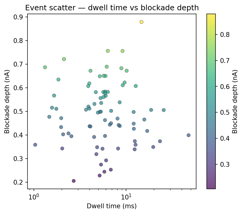
Scatter plots

A scatter plot of dwell time versus blockade depth is the standard visualization for nanopore translocation data:

import matplotlib.pyplot as plt

fig, ax = plt.subplots()
ax.scatter(df["duration"] * 1000, df["blockade_depth"], s=20, alpha=0.6)
ax.set_xlabel("Dwell time (ms)")
ax.set_ylabel("Blockade depth (nA)")
ax.set_xscale("log")
plt.show()

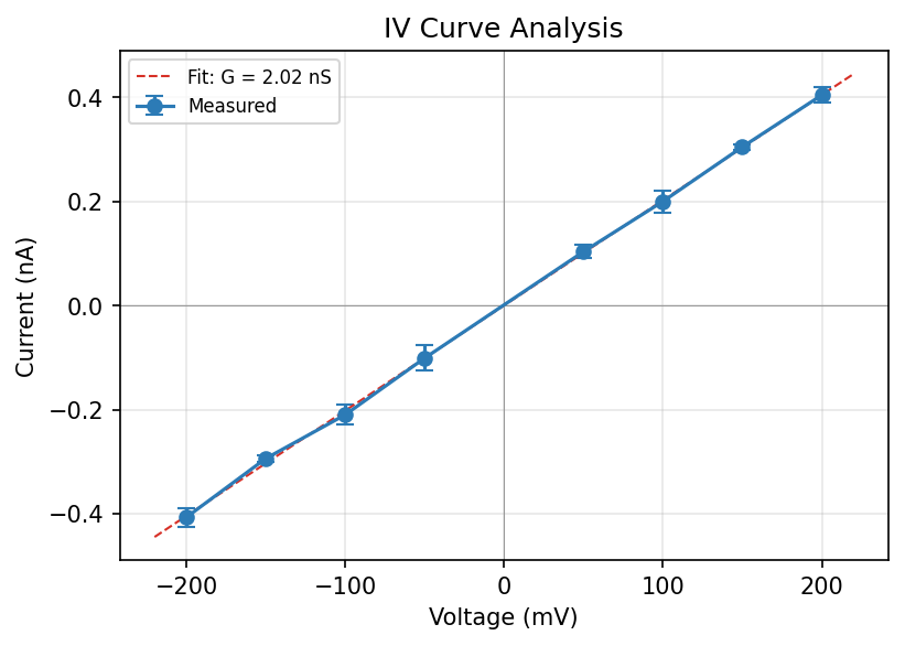
IV curve analysis

For recordings with multiple voltage steps, you can build a current–voltage curve:

Step 1: Extract mean current per voltage step:

vsteps = trace.traverse_to_rank("vstep")
voltages = []
currents = []
for vs in vsteps:
    v = vs.get_feature("voltage")
    voltages.append(v * 1000)   # convert to mV
    currents.append(vs.mean)

Step 2: Fit and plot:

import numpy as np
import matplotlib.pyplot as plt

coeffs = np.polyfit(voltages, currents, 1)
conductance_nS = coeffs[0] * 1000
print(f"Conductance: {conductance_nS:.2f} nS")

fig, ax = plt.subplots()
ax.plot(voltages, currents, "o", label="Measured")
fit_v = np.linspace(min(voltages), max(voltages), 100)
ax.plot(fit_v, np.polyval(coeffs, fit_v), "--", label=f"G = {conductance_nS:.1f} nS")
ax.set_xlabel("Voltage (mV)")
ax.set_ylabel("Current (nA)")
ax.legend()
plt.show()

Using IVCurveAnalyzer:

from ionique.parsers import IVCurveAnalyzer

analyzer = IVCurveAnalyzer(
    current=trace.current,
    parent_segment=trace,
    sampling_frequency=trace.sampling_freq,
    method="simple",
)
iv_data = analyzer.analyze()
# {voltage: (mean_current, std_current), ...}